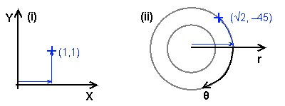
The two main types of coordinate system in 2D: (i) Cartesian, and (ii) polar. The blue point is at the same location relative to the origin but indexed differently.
3D display and interaction is an important part of modern computer systems. The most obvious example is in the game industry, where almost every game published in the 21st century has a 3D world, but 3D graphics are also important in business and science for data visualisation.
There are well documented libraries that allow you to use 3D graphics within your application (in particular DirectX and OpenGL, which interact with your graphics card for extra speed), and if you're using these you don't need to know everything about how 3D works. However, it's still a good idea to understand the principles in this article, even if you don't have to write the code that implements much of it. In some cases (for example if you're writing web games that run in a sandbox, or writing for a mobile or embedded device), these libraries might not be available and you will have to find or create the toolkit as well.
The purpose of this article is to introduce and explain the concepts behind 3D graphics and modelling, and not particularly to provide working code samples. If you read and understand everything within it you should be in a position to implement or use a 3D toolkit.
Dealing with a 3D world requires some mathematical knowledge, and there is little point attempting to read this article if you do not have it – instead, you should read up on it and understand it, and then return here. The two most important pieces of knowledge are an understanding of vector and matrix mathematics (specifically, dot and cross products, normalisation and matrix multiplication).
It may seem to be simple if you come from a computer graphics background, but even in two dimensions there are several choices of coordinate system. Firstly, there are two main types of system: a Cartesian system, where there are two linear axes at right angles to each other (usually called X and Y); and a polar system, where the axes are radius (r) and angle (θ).
The two main types of coordinate system in 2D: (i) Cartesian, and (ii) polar. The blue point is at the same location relative to the origin but indexed differently.
The Cartesian system has several advantages for use in computer graphics (not least that the pixels on the physical device are arranged in a Cartesian fashion, and also that the coordinate system is uniform through all space). Except for a very few specialised situations, you will have seen Cartesian systems, and it is by far the most common.
However, even within a system there are several choices. If you are coming from a computer graphics background, you will have notice that I have drawn what you may consider to be an 'upside down' Cartesian system – a mathematician would perhaps not even have noticed the Y axis being the 'right' way. There is also a choice of which axis is the primary axis (i.e. indexed first) – but for all standard situations there is only one choice there (X primary, i.e. indexers are [X,Y]). The choice of the right-handed X right, Y up that I have drawn, and the X right, Y down used by others, is arbitrary and you can choose either one.
I discuss 2D coordinate systems to demonstrate the choices that must be made whatever your dimensionality, and those that are often made for you without you knowing. In 3D there are similar choices to be made, but now there are three common types of coordinate system as opposed to just two:
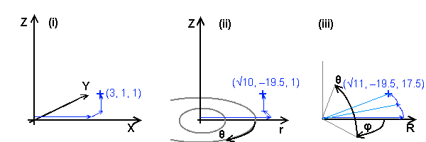
The three main types of coordinate system in 3D: (i) Cartesian X,Y,Z, (ii) cylindrical polar r,θ,Z, and (iii) spherical polar R,φ,θ. Again, the blue point is at the same location relative to the origin but indexed differently.
For similar reasons to 2D, a Cartesian system is most useful in most situations, although there are certain situations where the other two are useful (for example a planetary system or some areas of a magnetic field). I will use Cartesian coordinates through this article because the uniformity of coordinates through space is essential for using transformation matrices (see below), so I won't go into detail on the other two systems; if you are interested you can research them (you are online after all!).
As with 2D, there are also choices to be made about which way the axes lie. There are two main standards, both 'right-handed' with X as a horizontal axis (to the right): Z-up, Y-in, as I have drawn here; and Y-up, Z-out. Once again, the choice of which you choose to use is arbitrary. I will use a Z-up coordinate system throughout this article (and indeed others which I may have written about this subject).
With a point, a simple location vector (of the same dimension as the coordinate system) is enough to uniquely identify it. However, once you have more complex objects, you need to know more than simply where the origin of the object is. For example, in 2D you would typically specify an object's translation (the position of the origin) and also a rotation. These two elements are enough to uniquely define a non-deformational transformation (i.e. the object is the same shape and size as it began) in 2D, although for other (deformational) transformations, other elements may be necessary (scale factors, skew coefficients).
An object has its own local coordinate system, which is also transformed in the same way as the visual object. You can imagine a set of coordinate axes being attached to the graphical object and translated, rotated, skewed and scaled along with it. In this article I will deal solely with non-deformational transformations, specifying how objects are located and oriented within space, but the same principles apply if you want to modify your objects.
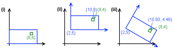
Non-deformational transformations and local coordinates in 2D. (i) The object to be transformed (blue rectangle and green inner square); (ii) The object and its axes (blue arrows) after translation; (iii) after rotation about the new origin. See text for details.
In the example above, the object is a blue rectangle 10 units by 5, with an inner green rectangle at local coordinates (8,4). When we translate the object to (2,5), the global coordinates of the green rectangle change accordingly, and the coordinate axes of the blue object are now centred at (2,2) in global space, but still align with the global axes. Under rotation (by 30°), the local coordinate axes no longer align with the global ones, and the global coordinates of the green rectangle (which is always at (8,4) locally) must now be determined using trigonometry.
The transformation, and in fact any transformation (including deformational ones), can also be represented in a Cartesian system as a transformation matrix. In 2D the matrix for a non-deformational transformation (rotation and translation) looks like this:
| ( | cos θ | sin θ | ty | ) |
| -sin θ | cos θ | ty | ||
| 0 | 0 | 1 |
... where θ is the angle of rotation, and (tx, ty) is the translation vector. (This would be a good point to mention that if you don't understand matrix mathematics, you should read up on it.) This matrix is equivalent to two equations to find the global coordinates of a local point:
X = (cos θ) x + (sin θ) y + ktx
Y = (-sin θ) x + (cos θ) y + kty
... with k being 1 for position vectors (i.e. points in space), and 0 for direction vectors (i.e. a difference between two points). For our green rectangle at (8,4) with a rotation of 30° and a translation of (2,5), we get:
X = (˝√3)×8 + ˝×4 + 2 = 4 + 4√3 = 10.93
Y = (-˝×8) + (˝√3)×4 + 5 = 1 + 2√3 = 4.46
... or equivalently:
| ( | ˝√3 | ˝ | 2 | )×( | 8 | )=( | 10.93 | ) | |
| -˝ | ˝√3 | 5 | 4 | 4.46 | |||||
| 0 | 0 | 1 | 1 | 1 |
... k being 1 for the location of the green rectangle, which is a point in the blue rectangle's space.
In 2D the matrix may not seem to give you much; it is easy enough to find the coordinates and target direction of objects with simple trigonometry, and it may seem simpler not to use the matrix – at least if you are not using deformational transformations. There is a certain amount of truth in this, in 2D, where there is only one angle to consider, although using a transformation matrix does have one major benefit: the inverse of the matrix will convert global coordinates to local ones. Inverting a matrix can be slow, however, and I will show a better way of finding local coordinates.
(Note: If the green object had a rotation (it has a translation, the (8,4) of its origin), and we were interested in points within it, we would need to multiply them by the green transform matrix and then by the blue one in order to determine their world coordinates – that is, an object's global transform matrix can be found by multiplying together all the matrices of its tree of parents. More on this later.)
In 3D the unique specification for a non-deformational transformation requires three different angles: yaw, pitch and roll. These three angles together are also called the Euler angles and together define an object's orientation within free space. Similar equations to those above for 2D can also be constructed for 3D, but they are significantly more complicated due to the interaction of the three angles, and converting from one coordinate space to another becomes more difficult, and also slow if done in volume due to the large number of trig functions required.
Instead, we can visualise the problem in a different way. Returning to the 2D transformation example from above, let us look at the principle axes (x,y) of the blue rectangle after rotation. The local axis x now points along (cos θ,-sin θ), and the local y along (sin θ,cos θ). (In fact, if you know one of these, the other can be found trivially due to their orthogonality – being at right angles to each other.) If you inspect the transformation matrix, you will see that the local x axis matches the first column, and the local y axis the second column. This is a general feature of a transformation matrix, which can be generally written:
| ( | rx | ux | tx | ) |
| ry | uy | ty | ||
| 0 | 0 | 1 |
| ( | . | . | . | ) |
| r | u | t | ||
| . | . | . |
... with r and u being the local x and y axes (right and up), and t the translation vector as before. Axis vectors have a zero in the third row, as they are directions, and the translation vector has a one, as it is a position (recall the k factor above).
In 2D this way of looking at the problem is not particularly helpful, but the concept extends to 3D where it is more helpful. A 3D transformation matrix, which is a 4×4 matrix, can be generally written in a similar way:
| ( | rx | fx | ux | tx | ) |
| ry | fy | uy | ty | ||
| rz | fz | uz | tz | ||
| 0 | 0 | 0 | 1 |
| ( | . | . | . | . | ) |
| r | f | u | t | ||
| . | . | . | . | ||
| . | . | . | . |
The new vector f is the forward vector, along the local y axis; u is now the local z axis. (If you aren't using Z-up, then you may need to re-arrange the order of your axis vectors.) Knowing which direction your object is facing is likely to be more useful, and readily available, than the Euler angles, and its transformation matrix stores this information conveniently. The axis vectors (for a non-deformational transformation only) follow the relationships u=r×f, r=f×u and f=u×r (the × being the vector cross product), and all three should be of unit length (normalised); these relationships mean that if you adjust any one of the three, you should adjust at least one of the others to maintain the non-deformational nature of the transformation.
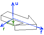
The principal axes of an object in 3D (right, forward and up), and a graphical representation of the local coordinates of a point
(Note: Some people prefer to store a non-deformational transformation in the form of an origin vector and a quaternion, which encodes a rotation in 3D. I prefer to work with matrices and will not mention quaternions again, but if you would like to research the other method then that term should open doors to you.)
As shown in the diagram, finding the local coordinates of a global point is graphically very simple: determine how far along each local axis the point is. (Remember that to go the other way, you simply multiply the position vector in local space by the matrix.) Fortunately, because the axis vectors are orthogonal, it is easy in practice too, without having to invert the matrix. The local coordinates of a point P are simply:
p = ((P-t).r, (P-t).f, (P-t).u)
... and you can take r, f, u and t out of the transformation matrix. (If you want the local equivalent of a direction vector, the calculation is the same but don't subtract t from it first.) Finding the local coordinates of one object in the space of another is a very common task (for example, determining if it is in range, or 'in front' of the other), and by using transformation matrices it becomes easy. It also makes our next task, projecting a 3D scene into 2D, much easier.
Projection is a general term to do with showing a set of points as they appear to another structure in space, but in the case of 3D graphics, it in practice means the process of taking 3D points, lines and surfaces and converting them to 2D in order to render them on the screen.
The first part of projection is something we have already done: transforming the points of the scene into 'camera space', the local coordinate system of the camera. The camera is an ordinary 3D object within your scene, with a transformation matrix containing its r, f, u and t vectors, which means you can orient and place it in any way that suits your needs, and you can use the dot product method to find the local coordinates of all points in the scene. (The camera's global transform is sometimes known as the worldview matrix.)
Once you have the points in the camera's local space, you must decide how to project them into 2D. The simplest approach is isometric – simply use the X and Z coordinates of the points, perhaps multiplied by a constant factor, as the screen coordinates (after filtering out points behind the camera). An isometric view gives you no distance information, although you can still perform depth sorting (see later) so it is only suitable when all the elements of the scene are at a similar distance – and if you want an isometrically rendered game, chances are that it is overkill to use a fully 3D model for the mechanics.
Another approach is to use the distance as a scaling factor: the projected coordinates are [x÷y, z÷y], again multiplied by a constant scale factor dependent on the size of your viewport. This method works well for small fields of view, for example in an embedded flash game or a small data visualisation panel; as the angle to a point increases, so does the distortion (shapes become 'stretched' away from the centre of the view), and it is not possible to show a field of view of 90° or more this way. To present a good, undistorted image a f.o.v. of less than ±30° (60° in total) is advisable.
The most correct approach is to use the trigonometric functions to find the angles of each point relative to the camera. Effectively, this is performing a coordinate transformation from the Cartesian space in which we have been working to a spherical polar space, and the projected coordinates become [atan2(x, y), atan2(z, √[x˛+y˛])]. This approach allows you to have a full surround field of view (±180° horizontally, ±90° vertically), although a f.o.v. of more than about ±80° looks strange unless you have a wraparound monitor.
For a normal user, even at full screen a monitor will be at most 30°, so for a non-distorting full screen view, you should use ±15° or so. However, most gamers at least will have become used to playing with a wider field of view, perhaps as much as ±90° for a first-person full screen game.
The final step is to convert your resulting 2D Cartesian coordinates to screen space. Typically this means you need to add a fixed amount to both X and Y in order to centre the projected image in the viewport, and in most environments you will also have to reverse the Y axis, as the projected Y is upwards and most computer graphics environments use Y-downwards.
For reference, here's an implementation of a 1/y projection (this one's in ActionScript, taken from my Flash library, but the code is simple enough to adapt to other conventional languages). You won't be able to simply copy and paste it unless your vector and transformation matrix classes are the same as mine, but it should show you how to write one that suits you.
public function ProjectMultiple(worldCoordsA:Vector.<Vector3>, ctm:Matrix = null) : Vector.<Vector3> {
var ra:Vector.<Vector3> = new Vector.<Vector3>(worldCoordsA.length);
if (ctm) worldCoordsA = ctm.TransformMultiple(worldCoordsA);
if (!lastTransform) lastTransform = GlobalTransform;
ra = lastTransform.WorldToLocalMultiple(worldCoordsA);
for (var i:int = 0; i < worldCoordsA.length; i++) {
var r:Vector3 = ra[i];
var z:Number = r.y;
r.y = -r.z; // Y reversed for top-down window coords
r.z = z;
if(z > threshold){
r.w = baseline / z; // Absolute scale factor
} else {
// Linear extrapolation of near-field distortion; allows interpolation
// of projected lines with one endpoint in the backfield with reasonable accuracy
var oneovert:Number = 1 / threshold;
r.w = (baseline * oneovert) + ((0.1 - z) * baseline * oneovert * oneovert);
// (b/z0) + (z0-z)(b/z0˛) for z0 = 0.1
}
r.rw = r.w * omag / baseline; // Relative scale factor
r.x *= r.w; r.y *= r.w;
}
return ra;
}
In this article I've explained the concepts and techniques needed to visualise, create and project points in three dimensions, and introduced the idea of transformation matrices, local coordinates and how to transform between local and global coordinates (and vice versa). In the second part, I'll show how to deal with lines and surfaces, diffuse lighting and creating solid-looking objects.